Example code for loading and analyzing sample audio file – Exploring Audio Data

Before diving into audio data analysis with Librosa, you’ll need to install it. To install Librosa, you can use pip, Python’s package manager:
pip install librosa

This will download and install Librosa, along with its dependencies.

Now that you have Librosa installed, let’s begin by loading an audio file and performing some basic analysis on it. In this example, we’ll analyze a sample audio file. We can read audio files using SciPy as follows:
from scipy.io import wavfile
import matplotlib.pyplot as plt
sample_rate, data = wavfile.read(‘cat_1.wav’)
print(sample_rate)
print(data)
Visulize the wave form
plt.figure(figsize=(8, 4))
plt.plot(data)
plt.title(‘Waveform’)
plt.xlabel(‘Sample’)
plt.ylabel(‘Amplitude’)
plt.show()

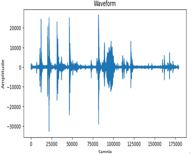
We get the following result:

Figure 10.1 – Waveform visualization

The provided code is for loading an audio file in WAV format, extracting information about the audio, and visualizing its waveform using Python. Here’s a step-by-step explanation of the code.

Importing libraries

from scipy.io import wavfile: This line imports the wavfile module from the scipy.io library, which is used to read WAV audio files.

import matplotlib.pyplot as plt: This line imports the pyplot module from the matplotlib library, which is used for creating plots and visualizations.

from IPython.display import Audio: IPython.display’s Audio module allows audio playback integration within Jupyter notebooks.

Loading the audio file

sample_rate, data = wavfile.read(‘cat_1.wav’): This line loads an audio file named cat_1.wav and extracts two pieces of information:

• sample_rate: The sample rate, which represents how many samples (measurements of the audio signal) are taken per second. It tells you how finely the audio is represented.
• data: The audio data itself, which is an array of values representing the amplitude of the audio signal at each sample.

Printing sample rate and data

print(sample_rate): This line prints the sample rate to the console. The sample rate is typically expressed in hertz (Hz).

print(data): This line prints the audio data, which is an array of amplitude values sampled at the given sample rate. The printed data may look like a long list of numbers, each representing the amplitude of the audio at a specific point in time.

Visualizing the waveform

plt.figure(figsize=(8, 4)): This line sets up a new figure for a plot of a specified size (8 inches in width and 4 inches in height).

plt.plot(data): This line creates a line plot of the audio data. The x axis represents the sample index (time), and the y axis represents the amplitude of the audio at each sample. This plot is called the waveform.

plt.title(‘Waveform’): This line sets the title of the plot to Waveform.

plt.xlabel(‘Sample’): This line labels the x axis Sample, indicating the sample index.

plt.ylabel(‘Amplitude’): This line labels the y axis Amplitude, indicating the intensity or strength of the audio signal at each sample.

plt.show(): This line displays the plot on the screen.

The resulting visualization is a waveform plot that shows how the amplitude of the audio signal changes over time. It’s a common way to get a visual sense of the audio data, allowing you to see patterns, peaks, and troughs in an audio signal.

Let us plot the audio player:
   Audio player
    audio_player = Audio(data=data, rate=sample_rate)
    display(audio_player)

We have loaded audio data and extracted two pieces of information (sample rate and data) from an audio file. Next, let us see how to extract other important properties from audio data.